A large part of my work the past decade has involved applications of ecosystemic programming. I was introduced to the concept of musical ecosystems by Agostino Di Scipio’s lectures on his Audible Eco-Systemic Interface (AESI) project at the Centre de Creation Musicale Iannis Xenakis (Di Scipio, Lectures; Sound p.272). His approach to interactive electronic music suggested to me an elegant means of applying theories of kinetic art to sound and exploring the spatial diffusion of sound.
Ecosystems
An ecosystem is an autonomous system, which may be composed of nested autonomous systems: “units that hold their ground by moving in their environments according to their inherent laws” (Nees p.42). These ‘inherent laws’ govern behavior in reaction to changes in the environment. Autonomous systems can effect change in their environment, to which other systems (and they themselves) will react. The relationship systems have to each other and their environment — how they react to and influence each other — is called structural coupling. Inherent in all autonomous systems is the notion of competition between their constituent elements which, based on their structural coupling, leads to self-organization (Nees p.43). This self-organization often results in a balance being found between all of the elements. This balance may be tenuous and dynamic, and depending on environmental changes, lost and found again in a similar or dissimilar form and manner.
Applying the interrelations of an ecosystem as a model for music composition constitutes an ecological approach to composition in which “form is a dynamic process taking place at the micro, meso and macro levels. [It] is not defined by the algorithmic parameters of the piece but results from the interaction among its sonic elements” (Keller p.58). Form and structure are intimately tied to the ambience of the actual space the music occurs in. The computer, based on its programming, is structurally coupled with the environment via sound.
In ecosystemic music, change in the sonic environment is continuously measured by Kyma with input from microphones. This change produces data that is mapped to control the production of sound. Environmental change may be instigated by performers, audience members, sound produced by the computer itself, and the ambience of the space(s) in general. “[The] computer acts upon the environment, observes the latter’s response, and adapts itself” (Di Scipio, Sound p.275).
Ecosystemic Programming in Kyma
I have included some example Sounds that can be downloaded here. The starting point for me was to create a Sound in Kyma that I could program to behave as an independent object in a sonic environment. I began by taking an oscillator and programming it to limit its output in response to increased amplitude in the environment — a ducking patch. Programming this behavior involves amplitude tracking, which can be implemented in several ways. Example Sound A.1) Stereo Amp Limiting presents the core starting point for my approach to ecosystemic programming.

One of the signal paths leading to the final Mixer is the AEIOU OSC oscillator, the sound source (object) to be limited. The other signal path tracks amplitude data from a single audio input. I am using an Amplitude Follower (for computational economy) with a rather short TimeConstant (in order to have higher resolution of data). The Amplitude Follower averages the value of its samples, but this data still needs to be processed in order to generate control data for my purposes.
A comb Delay is next in the signal path. I prefer the results of a comb delay over an allpass delay, but I don’t believe there is a functional reason to avoid the use of an allpass filter. The delay fulfills a few needs at this point. First, I use a very small delay time and a very high Feedback setting to further average the signal coming from the Amplitude Follower. The high Feedback also increases the overall level of the signal being generated, which is necessary at some point in the signal path before converting it to a global controller.
The DelayScale parameter value fractionalizes the already small delay time. This parameter allows me to smooth out the response of the signal being generated. Smaller values produce more jittery results. Larger values — essentially a larger window to be averaged — smooth out the results. This control has proven to be critical to managing ecosystemic behavior. Fine-tuning the setting allows for many small attacks to synergistically equal a single large attack.
The final Sound in this path is a silent SoundToGlobalController, which converts the processed data stream into the EventValue labeled !Limit. The data coming from Delay is DC, on a scale of zero to one (0,1). It is mapped linearly to generate the value for !Limit. Graphing the possible output value (x) based upon the input value (y) produces a straight line of input = output.
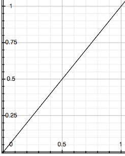
!Limit, where input = output
!Limit is used in the Mixer to inversely manage the value of the Left and Right channel outputs, as part of the formula (1 - !Limit). As the amplitude in the environment increases (as measured by the Amplitude Follower), it generates a higher value for !Limit, which results in an ultimately lower value for the Left and Right parameters in the Mixer output. If we graph the possible values we see:

(1 – !Limit)
This inversely related data could as easily have been generated in the SoundToGlobalController by placing the formula in the Value parameter as (1 - ([Delay] L)). By mathematically modifying the data in the Value parameter, we can modify the behavior of the object in simple but interesting ways. For example, the data ([Delay] L) can produce quadratic values by squaring it using this formula: (([Delay] L) ** 2). If we subtract that value from 1, we invert the values, so that the curve representing !Limit moves from one to zero as the tracked amplitude increases.
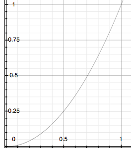
(([Delay] L) ** 2)

1 – (([Delay] L) ** 2)
Ultimately, programming more sophisticated object behavior will involve some mathematics to generate non-linear EventValues, combined with managing the sensitivity and smoothing of the sonic elements being tracked.
An alternative method of smoothing out the behavior of the data generated is now possible with the introduction of the LossyIntegrator Sound. This sound replaces the !Smooth function programmed into the DelayScale parameter. In the A.1) example, !Smooth increases the Delay time, which has the effect of smoothing out the averaging of the signal with larger delay times. The LossyIntegrator (see A.2) Stereo Amp Limiting alt Smooth) allows us to determine how long it will take for the output to decay to about 37% of the current value. In practice, the input (current value) is changing rather frequently. Because of this, the LossyIntegrator takes on the role of smoothing (or not) the behavior of the output as it moves towards one input value after another. While this introduces an additional Sound into the signal path, I am coming to prefer the output using the LossyIntegrator.

A critical point concerning the range of values for !Smooth is that if the Scale parameter in the LossyIntegrator is 0, the output will lock at the current value or jump to 0 (depending on the value in ReleaseTime). The solution is to program in a minimum value for !Smooth either in the VCS editor (such as 0.001) or to program it in the Scale and ReleaseTime parameters, e.g. (!Smooth + 0.001). Also, the values of Scale and ReleaseTime can be greater than 1, which is important to the extent to which change is smoothed out over time. I am using a maximum value of 10 in these example Sounds.
Having programmed a sound generating object to reduce its output as Kyma senses the amplitude in the environment increasing, it becomes an easy matter to program the sound to move in space in response to the amplitude tracking. B) Stereo Amp Panning demonstrates this. It is the same Sound as example A.2, however, I have changed the name of the GeneratedEvent from !Limit to !Angle, and if you examine the Left/Right fields in the Mixer, you can see that I have modified the formula. In example A.2, both fields are have 1 - !Limit determining their value. As !Limit increases, both Left and Right outputs decrease.

In example B, the Left field is 1 - !Angle, and the Right field is the inverse, simply !Angle. As the value for !Angle increases, the Left output value will decrease. Simultaneously, the Right output value will increase. This will create the perception of linear panning (from Left to Right).

Example B) Stereo Amp Panning

From these basic principles of feedback-based behavior, much more interesting and sophisticated behaviors can be programmed. The next step in the process is moving from a stereo to a multichannel environment. Future considerations will include tracking data other than amplitude, ecosystemic control of timbre, non-linear diffusion, asymmetrical speaker arrangements, microphone selection, microphone placement, and input mixing.
Bibliography
Di Scipio, Agostino. Lectures on eco-systemic music presented at Centre de Creation Musicale Iannis Xenakis (CCMIX) Summer Intensive, Alfortville, France. 6-7 July 2004.
Di Scipio, Agostino. “Sound is the Interface: from Interactive to Ecosystemic Signal Processing.” Organised Sound 8.3 (2003): 269-77.
Keller, Damián. “Compositional Processes from an Ecological Perspective.” Leonardo Music Journal 10 (2000): 55-60.
Nees, Georg. “Growth, Structural Coupling and Competition in Kinetic Art.” Leonardo 33.1 (2000): 41-7.