I’ve been interested in data-driven music over the past few years, and have explored this topic in some of my previous work (San Giovanni, Carbonfeed, #Ferguson) and I am currently working on a sound installation using historical data sets of California’s water history. Needless to say, data streams and CSV files have filled my computer screen more than I’d like to count (insert your favorite “If I had a nickel…” joke here). Wanting to integrate my data, in particular CSV data, with Kyma directly, without first modifying my information inside some other program is the reason behind this article/tutorial. I didn’t want to take some side road, spitting values to Kyma via OSC (requiring an external software), or taking a reductionist approach by compressing the data into single values. No, the point here is to step through all the data, line-by-line, using the values as they come in. Hence, today’s foray into CSV [comma-separated values] files.
This article is set it up much like how I learned, walking through the process step-by-step. Afterward, my hope is that you’ll have:
- a new tool to use (CSV files integration with Kyma)
- more confidence in scripting with Capytalk
- the ability to squeeze more “sound” from your data
First, you’ll need the walk-through Kyma files from the Kyma Community Library.
A note about the files. The walk-through is additive. That is, each step in the process is a new Sound, built upon the last. Feel free to jump to any point in the process, or go ahead and use your own CSV file with the Sounds. For the purpose of keeping things simple, the example CSV file is just a single column file with one number per line. This will help us keep us focused on the musical possibilities and working with Capytalk to help us get there. (The next post will delve into multi-column CSV and TSV [tab-separated values] files).
Overview
Step 0. Read a single column of a CSV file, line-by-line, and display its value
Step 1. Map values to pitch
Step 2. Morphing Timbre
Step 3. Exponentially Mapping Morph values
Step 4. Mapping Velocity
Step 5. Mapping Duration
Step 6. Match KeyDown with Duration
Step 7. Adding Pitch class
Step 8. Adding Register to Pitch Class
Step 9. Mapping Pan
Step 10. Correcting Pan Control
Step 0. Read in CSV data line-by-line
Inside the Kyma files, you’ll notice the “ReadingCSV.kym” file. Go ahead and open it. You’ll see one Sound (Text to Pitch90) and one Collection (Tutorial_StepByStep). All of today’s work is based off the Text to Pitch90 Sound, page 272 of Kyma X Revealed [which you can access from the Kyma 7 Help menu]. The original Sound converts character numbers (e.g. A=65) into pitches, and the Script moves character-by-character, resulting in a musical string phrase. The Sound provides a perfect set-up to read a CSV file, except that, instead of character-by-character, we’ll want to read our file line-by-line.
The example CSV file (sanfrandowntown_station23272_1990-2015_maxtemp.csv) is comprised of monthly max temperatures (in Fahrenheit) for Downtown San Francisco, every month from 1990 – 2015. 307 values in all.
For this initial step, let’s get familiar with the materials. Open up the Tutorial_StepByStep folder. You’ll notice all steps are separate Sounds. Go ahead and play the lineByline_step0_displayValue Sound. You should see a popup window displaying the first line of the CSV file. Click OK to view the next line of the CSV file, or go ahead and click Cancel to exit.

Step 0. Debug window displaying CSV line value
Before we move on, let’s get a basic understanding of what’s happening inside the script. And by understanding, I mean, we are only going to look at one line of code, as only one line of code stores the entire line of the CSV file into a variable.
Open up the Sound and inspect the Script parameter (Cmd-L for Large Window). Remember, all we want to do is alter the saving of variable from character to the entire line (a single CSV column). Thus, we change the original Text to Pitch90 Sound code from:
nbr := f next asInteger.
to…
nbr := f upTo: Character lf.
Kyma already had the code waiting for us to read CSV files! All we had to do was change one line. Notice how instead of converting f, the temporary character-by-character variable, to its ASCII number value, we collect all characters up to (upTo:) the end of line (Character lf).
Add in
self debugWithLabel: 'lineVal' value: nbr.
to take this collection of characters and spit them out as a popup display (debug:).
Step 1. Map Line Values to Pitch
This first step is effectively the same as the step 0, but now, we’ll get to hear the resultant sound rather than viewing numbers. The mapping differs from the original Text to Sound90 Sound in that instead of character-to-character pitch mapping (ASCII values), we are using the numbers (line-by-line) of our CSV file for our pitch mapping. For this step, all I did was remove the self debugWithLabel: line of code, and the script takes care of the rest!
Now, the walk-through could stop here. We’ve successfully integrated CSV files inside Kyma. High fives! But there’s more we could get out of these values. Do we really want to accept a random walk of pitches from 20-92 nn? (e.g. G#0 – G#6). What about controlling timbre, volume, duration, and location? As for controlling pitch, what if we wanted our CSV values to be based upon a musical scale? If you’re satisfied with CSV integration here, feel free to stop and start experimenting. Yet, if you’d like to continue to travel down the rabbit hole with me in getting more “sound” from your data, let’s move on to steps 2-10.
Step 2. Mapping Timbre (e.g. Morph)
Let’s take a look at timbre first. We have a “Morph” control on the GAOscillator in our example, so let’s use it! Inside the Script, you’ll notice a few things have changed.
A local variable has been added at the top:
| morphVal |
a new step inside the read file loop:
morphVal := (((nbr asNumber min: 100) / 100) max: 0).
and something new added to the MIDI keyDownAt: message:
timbre: morphVal
What does all this mean? First, we set up a variable at the top of the script named morphVal. Then, we assign our CSV value to the variable from inside the read file loop (line-by-line loop). Since our Morph parameter wants a value between 0-1, we need to normalize our nbr into a value between 0-1. With our normalized morphVal, we place this morph value inside the MIDI message and assign it to timbre (e.g. !KeyTimbre). If you’re asking how I knew how to use timbre:, I didn’t. I guessed. I got there by asking, “If velocity: X controls !KeyVelocity inside the MIDI event, what would control !KeyTimbre?” You guessed it! timbre: X. It works. Let’s listen!
I like that we have some morphing going on. Can’t hear it? Don’t believe me? Add this line [after the morphVal line] to see our normalized values in a debug window.
self debugWithLabel: 'lineValue' value: (((nbr asNumber min: 100) / 100) max: 0).
The code will stop every new line, and display the CSV nbr as a value between 0-1. min: and max: ensure a 0-1 range. This is what we want our morphVal to be. Yet, our values are high, averaging around the mid 60s (San Francisco is a warm place after all, just not in the summer). The mid-60s weather pattern normalizes into values of 0.60s, morphing our sound into the piano more than the harp. And I like the sound of the harp more than the sound of the piano! I’d prefer an exponential mapping, one that stays closer to the harp, but occasionally jumps into a morph of a piano.
Step 3. Nonlinear Mapping
On page 128 of Kyma X Revealed, there is a section on nonlinear faders. My code for this step borrows from this example.
nbrNorm := (((nbr asNumber min: 100) / 100) max: 0).

morphVal := nbrNorm into: #({0@0} {0.1@ 0.01} {0.6@0.05} {1@0.4}).
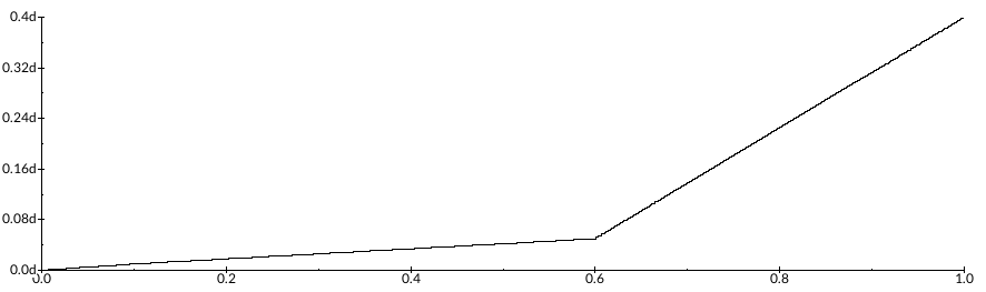
Step 3. Nonlinear mapping for Morphing
First, we reuse our normalization function and store this 0-1 value as the variable, nbrNorm. Then, we use into: to map our nbrNorm values onto a set of input@output pairs. In our example, 0 becomes 0, 0.1 becomes 0.01, 0.6 becomes 0.05, and 1 maps onto 0.4. All values in between are interpolated automatically. No additional coding required.
Listening to the example, we should hear more of the sound (0.6 values are the average) as more indicative of the harp timbre, with higher notes containing more timbral features of the piano. Why? Remember, a morph=0 contains only the harp timbre, and a morph=1 contains only the piano. Anything in between contains a percentage of both, like a sliding scale. The result is a shimmering/phase effect on higher pitches.
Step 4. Mapping Velocity
Pitch and timbre down. Let’s take a look at velocity (how hard a key is pressed). We’ll similarly, map velocity with the into: function.
veloVal := nbrNorm into: #({1@0.85} {0.6@0.52} {0.5@0.5} {0.4@0.52} {0@1}).

Step 4. Nonlinear mapping for Velocity
This non-linear mapping reveals to us that lower and higher notes will have a higher velocity (played louder), than the middle values (our majority of notes). The non-linear mapping places volume peaks onto less-played notes, offering moments of loudness.
Step 5. Duration
The Script currently sets every note to 1 beat, that is, 1 is our current duration value. Yet, what if we took our CSV number and used this to select from an array of durations?
| durIndex durVal |

durIndex := ((nbr asNumber rounded max: 20) mod: 4).

durVal := durIndex of: #(0.5 0.5 1 2).
In the script, we add two more variables, one to be the index pointer, and a second to become the duration value. ((nbr asNumber rounded max: 20) mod: 4) takes our value, rounds it to an integer, and with mod: returns an integer between 0-3. This 0-3 is a perfect index for an array of durations. With values for beats being 1=quarterNote, we can set up a simple duration array #(0.5 0.5 1 2) comprised of two eighth notes, one quarter note, and one half note.
Wait!? What?! That sounds the same! Yes, with the long note tail, it’s hard to differentiate between durations, so it sounds strikingly similar. Durations only account for the durations of the notes, not when the notes occur. To match duration with timing, we can use the same array, but we’ll need one more step.
Step 6. Matching Note Onset with Note Duration
We can reuse our duration array, but we’ll need to alter the original code a bit more. In the MIDI message, we notice keyDownAt: t beats. This tells us that t controls when the note is played, where t is the keyDown time. In the file read loop, the original script advances t by 1 with each new CSV value (since our values never go above 97).
(nbr asNumber < 97) ifTrue: [t := t + 0.25] ifFalse: [t := t + 1].
Since we want to make this t value advance by our own duration array, we can simply comment out or delete the original script’s function. I have commented out this line so you can see it, but feel free to delete.
Now, we’ll supplement our own advancement of t.
durVal := durIndex of: #(0.5 0.5 1 2).

t := t + durVal.
This matches timing and duration of notes, and now, we’ll definitely hear the difference.
Step 7. Pitchclass (musical scale)
Instead our file playing a “random” array of semitones from 20-92 (92 being our largest value in the CSV file), let’s condense our pitch choice into an array of notes from a scale. For the example, I chose an octatonic scale: #(0 1 3 4 6 7 9 10)
| pitchClass |

pitchClass := ((nbr asNumber max: 20) mod: 8) of: #(0 1 3 4 6 7 9 10).
inside the MIDI keyDownAt: message
frequency: (pitchClass + 60) nn
We again use our CSV value (nbr) to select pitch. Except this time, we mod: the result and pick a pitch class. With our pitch class in hand, we’ll add this by 60 (C4) to have our file play from within a C octatonic scale.
Step 8. Add Octave Register
Now that we have pitch classes happening, let’s add register back in to our notes. I like the high pitched elements, and I don’t want to get rid of them completely.
| register |

register := ((nbr asNumber max: 0) / 12) rounded.
inside MIDI keyDownAt: message
frequency: ((pitchClass + (12 * register)) max: 20) nn
Our script stores our CSV value (nbr) as a value representing octave register (something like 4, 5, 7), just like we would if talking about a pitch (e.g. C4, F5, G#7). We take the octave register and multiply by 12, since equal temperament is mod:12 arithmetic. We want to make sure we don’t get below 20 nn (low end of piano) so we add in a max: 20 safety net.
Step 9. Mapping Pan
Thus far, we’ve mapped a single CSV value onto pitch, timbre, velocity, duration, and timing. The final parameter of sound we’re missing here is location. Let’s place each sound in its own space within a stereo field using Pan.
Up until now, we’ve gotten away with mapping inside the MIDI message. Since pan is a separate Sound in Kyma, we’ll need one fancy line of code to help out. As reference, I found the help on page 274 of Kyma X Revealed.
self controller: !Panning setTo: 0.5 atTime: 0.

self controller: !Panning setTo: nbrNorm atTime: t beats.
With this, our script controls a HotValue, !Panning, and moves this pan control every t beats (from our duration control step). We use the normalized value (0-1) because the Pan Sound takes a 0-1 input to move the sound left-to-right. Inside the Pan Sound, we place !Panning in the Pan parameter field, and voila! Automatic pan control.
Step 10. Correcting Pan Control
Listening back, we have two problems. One, our average values are greater than 0.5, and as a result, lean toward the right speaker. Second, any negative, or 0, value in our CSV value cuts sound in the right speaker because of the hard 0 value attribute of the pan. Let’s rein in the sound toward the middle and fix our hard cut issues with our mapping into: {0@1} schema we’ve used before.
| panPos |

panPos := nbrNorm into: #({1@0.75} {0.6@0.52} {0.5@0.5} {0.4@0.3} {0@0.25}).

self controller: !Panning setTo: panPos atTime: t beats.
We take our normalized values and remap them toward the middle.
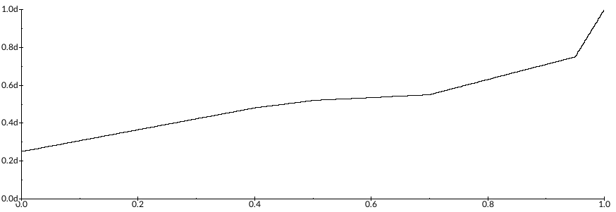
Step 10. Nonlinear mapping for Pan
As we can see in the envelope shape, most of our values remain in the center, with only extremely high values pushing toward the right speaker.
Closing
I hope by now, you’ve seen the possibilities with adding in, just a sprinkle, of Capytalk to organically modify a Sound. And we certainly have come a long way! We’ve systematically nabbed San Francisco’s temperature from a CSV file, and used these temperature values to dynamically change a sound! As you move ahead, and you find yourself lost, as I often do, just take it one step at a time, and don’t forget the debug: x command!
Here’s a short, 90 second exploration using the CSV file and Sounds above. Enjoy!
In my next post, we’ll take a look at multi-column CSV/TSV files, building upon our knowledge from this exercise.
Additional reference: if have a multi-column CSV file that you want to try these Sounds with, I highly recommend csvkit. It’s a simple library run from Terminal (for all you Mac users), works on Mac, Linux, and Windows and let’s you quickly manipulate csv files. I used it to create this example. Download and learn more at the csvkit website. Additionally, check out the Kyma Wave editor (File > New > Sample file), where you can transform your TSV file directly into a wavetable.
About the author.  Jon Bellona is an intermedia artist/composer who specializes in digital technologies. He has been working with Kyma since 2009.